과거 데이터 기반으로, 입력 주어졌을 때 출력(예측값)이 나와야 한다.
예측하고자 하는 변수 = target variable(타겟 변수)
타겟 변수가 실수이면 = regression problem,
타겟 변수가 카테고리 변수이면 = classification (대표적인 방법론: 로지스틱 회귀)
이 둘은 supervised learning(지도 학습)이다.
unsupervised learning(비지도 학습)에는 clustring(k-means) 등이 있다.
선형회귀 Linear Regression
- 종속 변수 𝑦와 한개 이상의 독립 변수 𝑋와의 선형 관계를 모델링(=1차로 이루어진 직선을 구한다)하는 방법론
- 최적의 직선을 찾아 독립 변수와 종속 변수 사이의 관계를 도출하는 과정
독립 변수= 입력 값이나 원인(input)
종속 변수 = 독립 변수에 의해 영향을 받는 변수(output)
<simple linear regression>(독립변수x가 1개일 때)


데이터를 가장 잘 설명하는 직선은 예측한 값이 실제 데이터의 값과 가장 비슷해야 합니다.
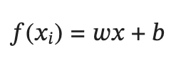
우리의 모델이 예측한 값은 위에서 알 수 있듯 𝑓(𝑥𝑖)입니다. 그리고 실제 데이터는 𝑦 입니다.
실제 데이터(위 그림에서 빨간 점) 과 직선 사이의 차이를 줄이는 것이 우리의 목적입니다.
그것을 바탕으로 cost function을 다음과 같이 정의해보겠습니다.
(n: 샘플 수, i: i번째 데이터)


우리는 cost function을 최소로 하는 𝑤와 𝑏를 찾아야 합니다.
이차함수이므로 이차함수의 최솟값을 구하는 방법은
1. 미분한 값이 0이 되는 지점찾기
[−3/2]
2. gradient descent
gradient descent
한번에 정답에 접근하는 것이 아닌 반복적으로 정답에 가까워지는 방법

fpnum = sympy.lambdify(w, fprime)2. 처음 𝑤 값을 설정한 뒤, 반복적으로 최솟값을 향해서 접근
w = 10.0 # starting guess for the min

for i in range(1000):
w = w - fpnum(w)*0.01 # with 0.01 the step size결과는 미분한 값과 같다
실제로 적용해보기 :
linear regression 방법을 사용해서 시간 흐름에 따른 지구의 온도 변화 분석
Global temperature anomaly라는 지표를 통해서 분석을 해볼 것입니다.
여기서 temperature anomaly는 어떠한 기준 온도 값을 정해놓고 그것과의 차이를 나타낸 것입니다. 예를 들어서 temperature anomaly가 양수의 높은 값을 가진다면 그것은 평소보다 따듯한 기온을 가졌다는 말이고, 음수의 작은 값을 가진다면 그것은 평소보다 차가운 기온을 가졌다는 말입니다.
세계 여러 지역의 온도가 각각 다 다르기 때문에 global temperature anomaly를 사용해서 분석을 하도록 하겠습니다. 자세한 내용은 아래 링크에서 확인하실 수 있습니다.
https://www.ncdc.noaa.gov/monitoring-references/faq/anomalies.php
Global Surface Temperature Anomalies | National Centers for Environmental Information (NCEI)
www.ncei.noaa.gov
Step 1 : Read a data file
NOAA(National Oceanic and Atmospheric Administration) 홈페이지에서 데이터를 가져오겠습니다.
아래 명령어로 데이터를 다운받고, numpy 패키지를 이용해 불러오겠습니다.
from urllib.request import urlretrieve
import numpy

URL = 'http://go.gwu.edu/engcomp1data5?accessType=DOWNLOAD'
urlretrieve(URL, 'land_global_temperature_anomaly-1880-2016.csv')

fname = '/content/land_global_temperature_anomaly-1880-2016.csv'
year, temp_anomaly = numpy.loadtxt(fname, delimiter=',', skiprows=5, unpack=True)
Step 2 : Plot the data
Matplotlib 패키지의 pyplot을 이용해서 2D plot을 찍어보도록 하겠습니다.
from matplotlib import pyplot
%matplotlib inline
pyplot.rc('font', family='serif', size='18')

#You can set the size of the figure by doing:
pyplot.figure(figsize=(10,5))

#Plotting
pyplot.plot(year, temp_anomaly, color='#2929a3', linestyle='-', linewidth=1)
pyplot.title('Land global temperature anomalies. \n')
pyplot.xlabel('Year')
pyplot.ylabel('Land temperature anomaly [°C]')
pyplot.grid();
Step 3 : Analytically
Linear regression을 하기 위해서 먼저 직선을 정의하겠습니다.
그 다음 최소화 해야 할 cost function은 다음과 같습니다.

이제 cost function 을 구하고자 하는 변수로 미분한 뒤 0이 되도록 하는 값을 찾으면 됩니다.

w = numpy.sum(temp_anomaly*(year - year.mean())) / numpy.sum(year*(year - year.mean()))
b = a_0 = temp_anomaly.mean() - w*year.mean()

print(w)
print(b)#0.01037028394347266
#-20.148685384658464
이제 그래프로 그려서 확인해보도록 하겠습니다
reg = b + w * year

pyplot.figure(figsize=(10, 5))

pyplot.plot(year, temp_anomaly, color='#2929a3', linestyle='-', linewidth=1, alpha=0.5)
pyplot.plot(year, reg, 'k--', linewidth=2, label='Linear regression')
pyplot.xlabel('Year')
pyplot.ylabel('Land temperature anomaly [°C]')
pyplot.legend(loc='best', fontsize=15)
pyplot.grid();
'머신러닝' 카테고리의 다른 글
| 다중 로지스틱 회귀 (소프트맥스 회귀) (0) | 2022.12.05 |
|---|---|
| 로지스틱 회귀 sklearn logistic regression iris python (0) | 2022.12.04 |
| [머신러닝4] Logistic Regression 로지스틱 회귀 pyhton (0) | 2022.11.30 |
| [머신러닝3] Multiple Linear Regression 다중선형회귀 python (0) | 2022.11.30 |
| [머신러닝2] Polynomial Regression python (0) | 2022.11.30 |